Spin simulations in Julia – Utz Research Group

Julia is a programming language designed for numerical and scientific computation. It combined the convenience of an interpreted scripting language with the efficiency of compiled ones like C, Fortran, or C++. The goal of this effort is to provide a very simple and lightweight infrastructure for quick, but accurate, quantum mechanical simulations of small spin systems. NMR.jl represents spin operators in a Hilbert basis formed from the Kronecker
products of the individual \(|\alpha\rangle, |\beta\rangle,\dots\) spin states. It uses sparse matrices wherever possible. In this way, simulations of up to ten spins 1/2 tend to run in a matter of minutes. Larger spin systems, up to about twenty spins or so, are possible, but require significant computational resources.

Here is an example of such a calculation. These commands are meant to be run either as a Julia script, line-by-line on the Julia command line, or, most usefully, as an IJulia notebook in a web browser. If you have not done so, install the current version of NMR.jl in your Julia environment by running the Julia command

Pkg.clone("https://github.com/marcel-utz/NMR.jl");

This will take a few moments. Once it’s done, you are ready to go.

First, we create a clean workspace and declare usage of the NMR modules SpinSim and PauliMatrix:

workspace();
using NMR.SpinSim;
using NMR.PauliMatrix;

Then, we need to define the properties of the spin system. In the present case, we are modelling hydroxy-ethyl propionate (HEP). The molecule looks like this:

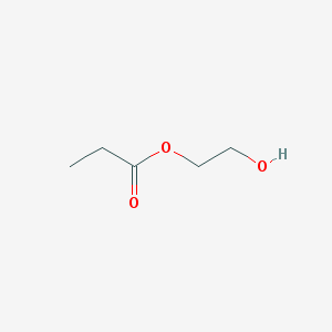
There are five protons on the propionate side, three methyl (a) and two methylene (b), and two pairs of methylene protons on the ethyl (right) side (c) and (d). We assume the hydroxyl proton to be in fast exchange with the solvent. In addition, there is a ¹³C label at the carboxylate site (x). Therefore, we are simulating a ten spin system overall.
The parameters are

Jaa=-12.4;
Jab=7.5;
Jax=7.2;
Jbb=-10.8;
Jbx=-5.6;
Jcc=-10.8;
Jcd=7.5;
Jcx=3.2;
Jdd=-12.4;
Jdx=1.7;
δa=1.25;
δb=4.15;
δc=2.3;
δd=1.8;

The Zeeman Hamiltonian (in the rotating frame) is defined by taking into account the chemical shifts of the protons and the Z component of the spin operators:

Hz=δa*(SpinOp(10,Sz,1)+SpinOp(10,Sz,2)+SpinOp(10,Sz,3))+
   δb*(SpinOp(10,Sz,4)+SpinOp(10,Sz,5))+
   δc*(SpinOp(10,Sz,7)+SpinOp(10,Sz,8))+
   δd*(SpinOp(10,Sz,9)+SpinOp(10,Sz,10)) ;

In addition, we need the J coupling Hamiltonian. We use strong coupling between chemically equivalent protons, and weak coupling in all other cases:

HJHHstrong=
2*pi*Jaa*(OpJstrong(10,1,2)+OpJstrong(10,2,3)+OpJstrong(10,1,3))+
2*pi*Jbb*OpJstrong(10,4,5)+
2*pi*Jcc*OpJstrong(10,7,8)+
2*pi*Jdd*OpJstrong(10,9,10);

HJHHweak=
2*pi*Jab*sum([OpJweak(10,k,l) for k=1:3,l=4:5])+
2*pi*Jcd*sum([OpJweak(10,k,l) for k=7:8,l=9:10]);

We also need some of the total spin operators, such as \(F_z\) and \(F_y\):

FzH=sum([SpinOp(10,Sz,k) for k=1:5])+sum([SpinOp(10,Sz,k) for k=7:10])
FyH=sum([SpinOp(10,Sy,k) for k=1:5])+sum([SpinOp(10,Sy,k) for k=7:10])
FmH=sum([SpinOp(10,Sm,k) for k=1:5])+sum([SpinOp(10,Sm,k) for k=7:10])
Fz=sum([SpinOp(10,Sz,k) for k=1:10])

Here, FzH is the \(F_z\) operator for the protons only, where as Fz applies
to all spins, including ¹³C.